1 词向量
因为我们的输入是一些文本,所以我们需要将这些文本转化为词向量。
- 如何加载训练好了的词向量
这里我们使用50维的向量来表示单词:
def read_glove_vecs(glove_file):
    with open(glove_file, 'r', encoding='utf8') as f:
        words = set()
        word_to_vec_map = {}
        for line in f:
            line = line.strip().split()
            curr_word = line[0]
            words.add(curr_word)
            word_to_vec_map[curr_word] = np.array(line[1:], dtype=np.float64)

        i = 1
        words_to_index = {}
        index_to_words = {}
        for w in sorted(words):
            words_to_index[w] = i
            index_to_words[i] = w
            i = i + 1
    return words_to_index, index_to_words, word_to_vec_map
word_to_index, index_to_word, word_to_vec_map = read_glove_vecs('data/glove.6B.50d.txt')
或者我们也可以使用w2v_utils中的库函数:
import w2v_utils
words, word_to_vec_map = w2v_utils.read_glove_vecs('data/glove.6B.50d.txt')
上面两种执行的结果是一样的。其中word_to_index代表的是每个单词对应的下标
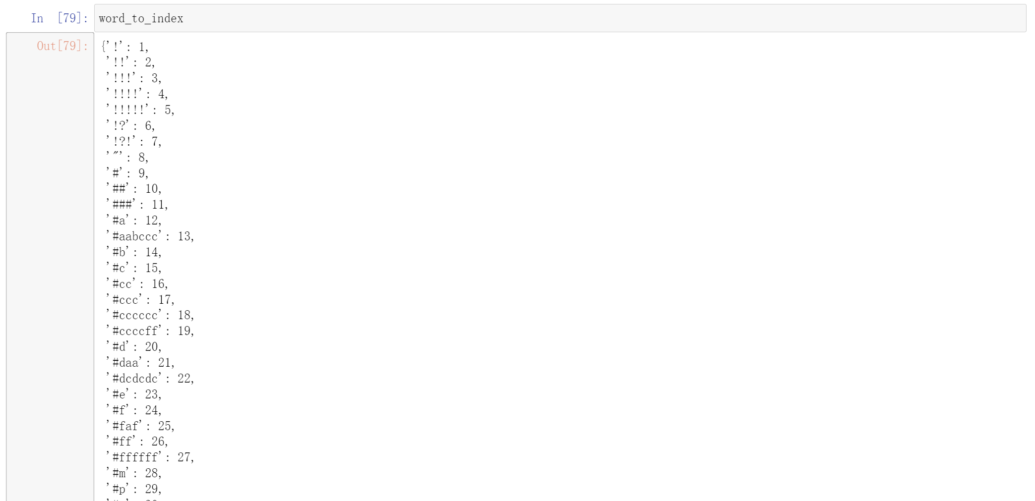
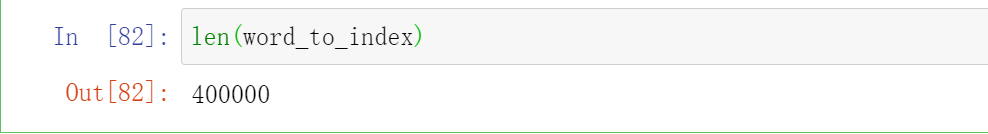
index_to_word是下表对应单词,其中一共有400000个单词
word_to_vec_map : 字典类型,单词到GloVe向量的映射
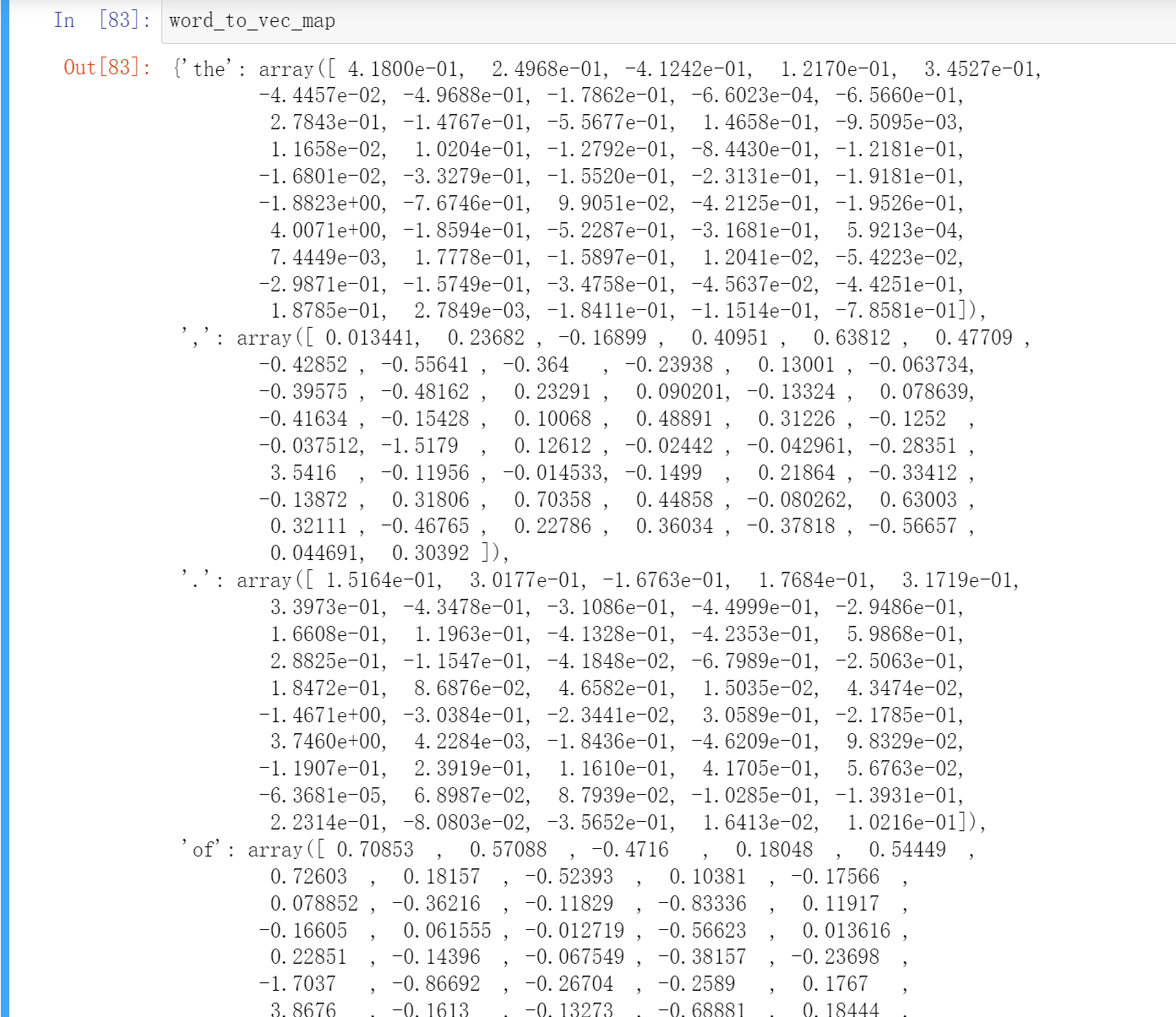
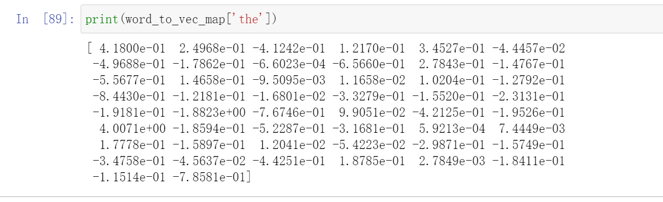
其中每一个单词都是50个数字表示
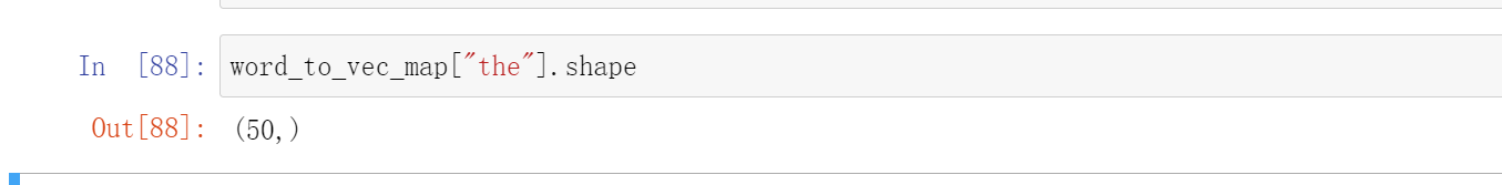
print(word_to_vec_map['the'])
因为独热向量不能很好地表示词语词之间的相似性,所以使用了GloVe向量,它保存了每个单词更多、更有用的信息,我们现在可以看看如何比较两个词的相似性。
1.1 余弦相似度
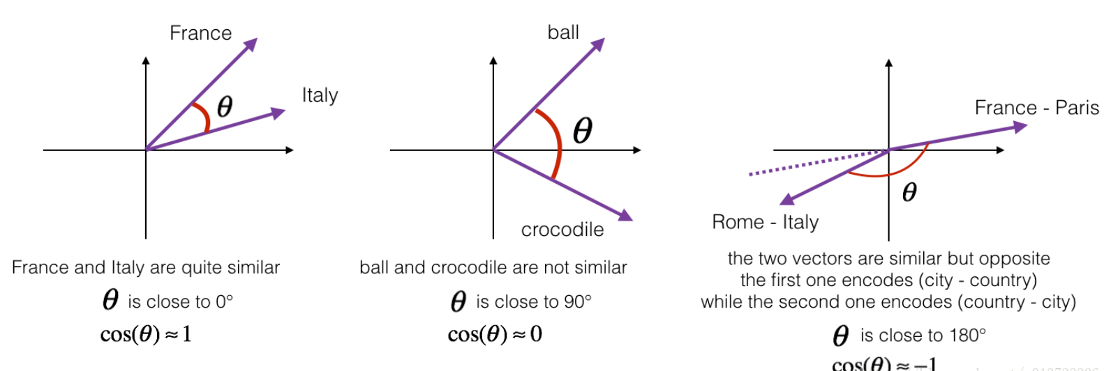
为了衡量两个词的相似程度,我们需要一种方法来衡量两个词的词嵌入向量之间的相似程度,给定两个向量\(u\)和\(v\),余弦相似度定义如下:
其中,\(u\cdot v\)是两个向量的点积(内积),\(||u||_2\)是\(u\)的范数(长度), \(\theta\)是\(u\)与\(v\)之间的夹角角度,\(u\)与\(v\)之间的相似度是基于他们之间的角度计算的,它们越相似,那么\(cos(\theta)\)的值就越接近于1;如果它们很不相似,那么他们的夹角就越大,\(cos(\theta)\)的值就越接近于-1。
接下来我们要实现一个计算两个词的相似度的函数cosine_similarity()
提醒:\(u\)的范数是这样定义的:\(||u||_2 = \sqrt{\sum_{i=1}^{n} u_i^2}\)
def cosine_similarity(u, v):
    """
    u与v的余弦相似度反映了u与v的相似程度

    参数:
        u -- 维度为(n,)的词向量
        v -- 维度为(n,)的词向量

    返回:
        cosine_similarity -- 由上面公式定义的u和v之间的余弦相似度。
    """
    distance = 0

    # 计算u与v的内积
    dot = np.dot(u, v)

    #计算u的L2范数
    norm_u = np.sqrt(np.sum(np.power(u, 2)))

    #计算v的L2范数
    norm_v = np.sqrt(np.sum(np.power(v, 2)))

    # 根据公式1计算余弦相似度
    cosine_similarity = np.divide(dot, norm_u * norm_v)

    return cosine_similarity
father = word_to_vec_map["father"]
mother = word_to_vec_map["mother"]
ball = word_to_vec_map["ball"]
crocodile = word_to_vec_map["crocodile"]
france = word_to_vec_map["france"]
italy = word_to_vec_map["italy"]
paris = word_to_vec_map["paris"]
rome = word_to_vec_map["rome"]

print("cosine_similarity(father, mother) = ", cosine_similarity(father, mother))
print("cosine_similarity(ball, crocodile) = ",cosine_similarity(ball, crocodile))
print("cosine_similarity(france - paris, rome - italy) = ",cosine_similarity(france - paris, rome - italy))
执行结果为:
cosine_similarity(father, mother) =  0.8909038442893615
cosine_similarity(ball, crocodile) =  0.27439246261379424
cosine_similarity(france - paris, rome - italy) =  -0.6751479308174201
当然你也可以随意修改其他的词汇,然后看看它们之间的相似性。
1.2 词类类比
在这里,我们将学习解决“A与B相比就类似于C与____相比一样”之类的问题,打个比方,“男人与女人相比就像国王与女皇相比”。实际上我们需要找到一个词\(d\),然后\(e_a, e_b, e_c, e_d\)满足以下关系:\(e_b - e_a \approx e_d - e_c\),当然,\(e_b - e_a\)与\(e_d - e_c\)是使用余弦相似性来做判断的。
def complete_analogy(word_a, word_b, word_c, word_to_vec_map):
    """
    解决“A与B相比就类似于C与____相比一样”之类的问题

    参数:
        word_a -- 一个字符串类型的词
        word_b -- 一个字符串类型的词
        word_c -- 一个字符串类型的词
        word_to_vec_map -- 字典类型,单词到GloVe向量的映射

    返回:
        best_word -- 满足(v_b - v_a) 最接近 (v_best_word - v_c) 的词
    """

    # 把单词转换为小写
    word_a, word_b, word_c = word_a.lower(), word_b.lower(), word_c.lower()

    # 获取对应单词的词向量
    e_a, e_b, e_c = word_to_vec_map[word_a], word_to_vec_map[word_b], word_to_vec_map[word_c]

    # 获取全部的单词
    words = word_to_vec_map.keys()

    # 将max_cosine_sim初始化为一个比较大的负数
    max_cosine_sim = -100
    best_word = None

    # 遍历整个数据集
    for word in words:
        # 要避免匹配到输入的数据
        if word in [word_a, word_b, word_c]:
            continue
        # 计算余弦相似度
        cosine_sim = cosine_similarity((e_b - e_a), (word_to_vec_map[word] - e_c))

        if cosine_sim > max_cosine_sim:
            max_cosine_sim = cosine_sim
            best_word = word

    return best_word
我们来测试一下:
triads_to_try = [('italy', 'italian', 'spain'), ('india', 'delhi', 'japan'), ('man', 'woman', 'boy'), ('small', 'smaller', 'large')]
for triad in triads_to_try:
    print ('{} -> {} <====> {} -> {}'.format( *triad, complete_analogy(*triad,word_to_vec_map)))
测试结果:
italy -> italian <====> spain -> spanish
india -> delhi <====> japan -> tokyo
man -> woman <====> boy -> girl
small -> smaller <====> large -> larger
现在词类类比已经完成了,需要记住的是余弦相似度是比较词向量相似度的一种好方法,尽管使用L2距离(欧式距离)来比较也是可以的。
2 Emoji表情生成器
在这里,我们要学习使用词向量来构建一个表情生成器。
你有没有想过让你的文字也有更丰富表达能力呢?比如写下“Congratulations on the promotion! Lets get coffee and talk. Love you!”,那么你的表情生成器就会自动生成“Congratulations on the promotion! ? Lets get coffee and talk. ☕️ Love you! ❤️”。
另一方面,如果你对这些表情不感冒,而你的朋友给你发了一大堆的带表情的文字,那么你也可以使用表情生成器来怼回去。
我们要构建一个模型,输入的是文字(比如“Let’s go see the baseball game tonight!”),输出的是表情(⚾️)。在众多的Emoji表情中,比如“❤️”代表的是“心”而不是“爱”,但是如果你使用词向量,那么你会发现即使你的训练集只明确地将几个单词与特定的表情符号相关联,你的模型也了能够将测试集中的单词归纳、总结到同一个表情符号,甚至有些单词没有出现在你的训练集中也可以。
在这里,我们将开始构建一个使用词向量的基准模型(Emojifier-V1),然后我们会构建一个更复杂的包含了LSTM的模型(Emojifier-V2)。
首先这里我们需要先安装pip install emoji
import numpy as np
from emo_utils import *
import emoji
import matplotlib.pyplot as plt
import pandas as pd
import tensorflow as tf
from tensorflow.keras import layers,Sequential
import tensorflow.keras as keras
%matplotlib inline
2.1 读取数据
data_train = pd.read_csv('data/train_emoji.csv',header=None)
data_test=pd.read_csv('data/test.csv',header=None)
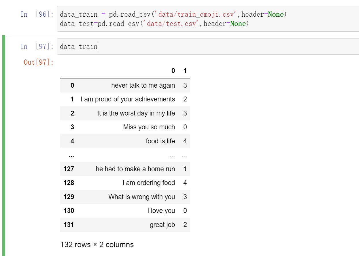
X:包含了127个字符串类型的短句
Y:包含了对应短句的标签(0-4)
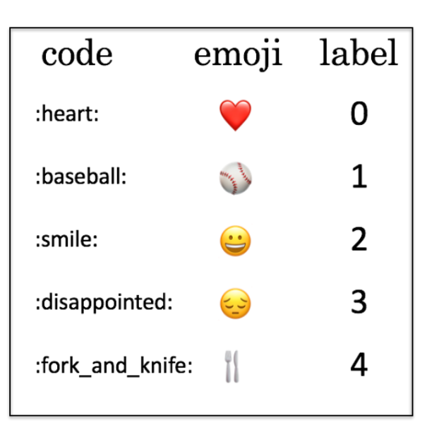
其中每个标签是这样的:
现在我们来加载数据集,训练集:127,测试集:56。
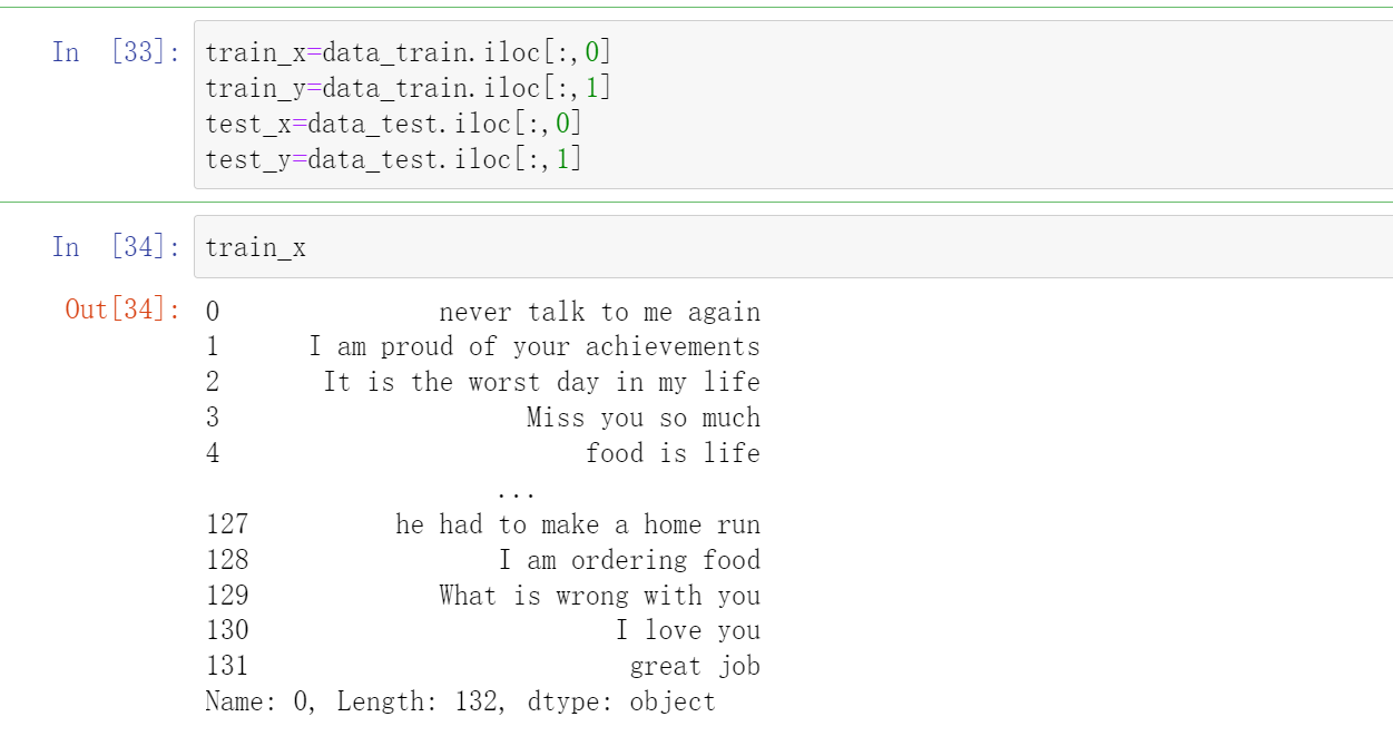
train_x=data_train.iloc[:,0]
train_y=data_train.iloc[:,1]
test_x=data_test.iloc[:,0]
test_y=data_test.iloc[:,1]

train_x
查看数据集中最长的句子的单词的个数
aa = max(train_x, key=len);
maxLen = len(max(train_x, key=len).split())
maxLen
# 10
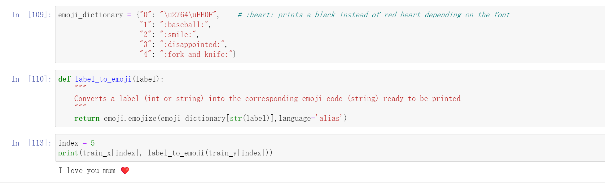
你可以随意更改index的值来看看训练集里面到底有什么东西
emoji_dictionary = {"0": "\u2764\uFE0F",    # :heart: prints a black instead of red heart depending on the font
                    "1": ":baseball:",
                    "2": ":smile:",
                    "3": ":disappointed:",
                    "4": ":fork_and_knife:"}
def label_to_emoji(label):
    """
    Converts a label (int or string) into the corresponding emoji code (string) ready to be printed
    """
    return emoji.emojize(emoji_dictionary[str(label)],language='alias')
index = 5
print(train_x[index], label_to_emoji(train_y[index]))
2.2 加载词嵌入
第一种:
def read_glove_vecs(glove_file):
    with open(glove_file, 'r', encoding='utf8') as f:
        words = set()
        word_to_vec_map = {}
        for line in f:
            line = line.strip().split()
            curr_word = line[0]
            words.add(curr_word)
            word_to_vec_map[curr_word] = np.array(line[1:], dtype=np.float64)

        i = 1
        words_to_index = {}
        index_to_words = {}
        for w in sorted(words):
            words_to_index[w] = i
            index_to_words[i] = w
            i = i + 1
    return words_to_index, index_to_words, word_to_vec_map
word_to_index, index_to_word, word_to_vec_map = read_glove_vecs('data/glove.6B.50d.txt')
或者我们也可以:
word_to_index, index_to_word, word_to_vec_map = emo_utils.read_glove_vecs('data/glove.6B.50d.txt')
word_to_index:字典类型的词汇(400,001个)与索引的映射(有效范围:0-400,000)
index_to_word:字典类型的索引与词汇之间的映射。
word_to_vec_map:字典类型的词汇与对应GloVe向量的映射。
2.3 模型预览
在这个部分中,我们会使用mini-batches来训练Keras模型,但是大部分深度学习框架需要使用相同的长度的文字,这是因为如果你使用3个单词与4个单词的句子,那么转化为向量之后,计算步骤就有所不同(一个是需要3个LSTM,另一个需要4个LSTM),所以我们不可能对这些句子进行同时训练。
那么通用的解决方案是使用填充。指定最长句子的长度,然后对其他句子进行填充到相同长度。比如:指定最大的句子的长度为20,我们可以对每个句子使用“0”来填充,直到句子长度为20,因此,句子“I love you”就可以表示为(\(e_I, e_{love}, e_{you}, \vec{0}, \vec{0}, \ldots ,\vec{0}\))。
- 嵌入层( The Embedding layer)
在keras里面,嵌入矩阵被表示为“layer”,并将正整数(对应单词的索引)映射到固定大小的Dense向量(词嵌入向量),它可以使用训练好的词嵌入来接着训练或者直接初始化。在这里,我们将学习如何在Keras中创建一个Embedding()层,然后使用Glove的50维向量来初始化。因为我们的数据集很小,所以我们不会更新词嵌入,而是会保留词嵌入的值。
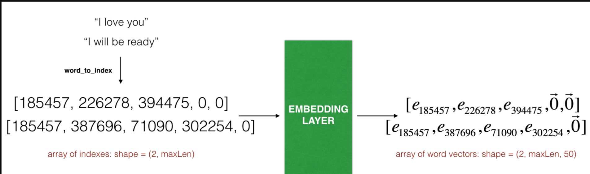
在Embedding()层中,输入一个整数矩阵(batch的大小,最大的输入长度),我们可以看看下图:
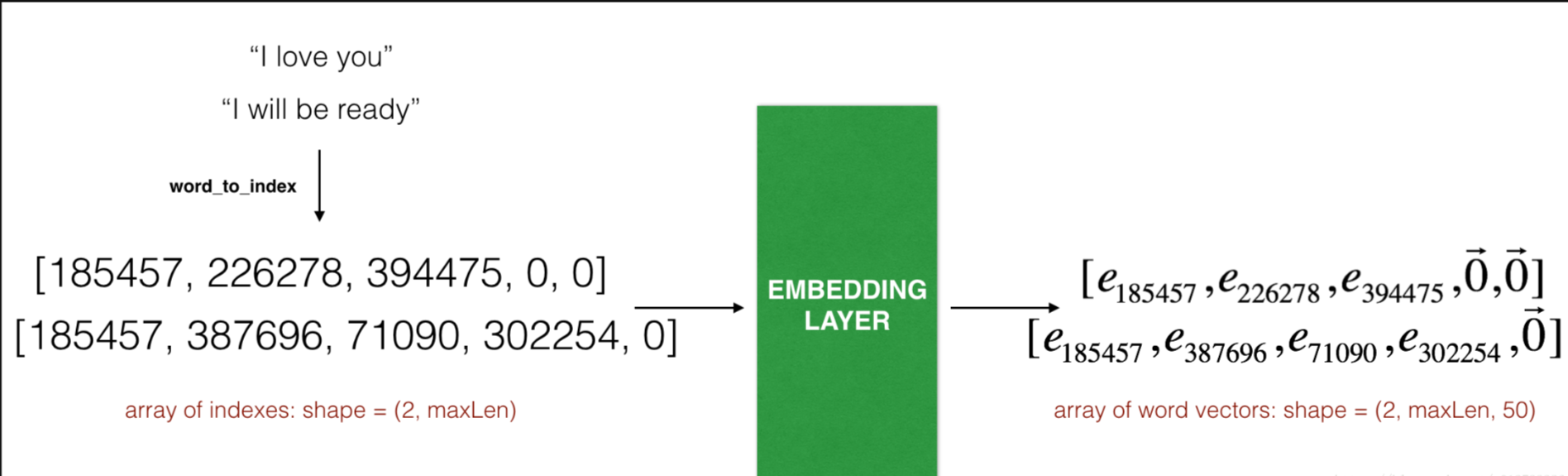
Embedding 层。这个例子展示了两个样本通过embedding层,两个样本都经过了max_len=5的填充处理,最终的维度就变成了(2, max_len, 50),这是因为使用了50维的词嵌入。
输入的最大的数(也就是说单词索引)不应该超过词汇表包含词汇的数量,这一层的输出的数组的维度为(batch size, max input length, dimension of word vectors)。
第一步就是把所有的要训练的句子转换成索引列表,然后对这些列表使用0填充,直到列表长度为最长句子的长度。
我们先来实现一个函数,输入的是X(字符串类型的句子的数组),再转化为对应的句子列表,输出的是能够让Embedding()函数接受的列表或矩阵
def sentences_to_indices(X, word_to_index, max_len):
    """
    输入的是X(字符串类型的句子的数组),再转化为对应的句子列表,
    输出的是能够让Embedding()函数接受的列表或矩阵(参见图4)。

    参数:
        X -- 句子数组,维度为(m, 1)
        word_to_index -- 字典类型的单词到索引的映射
        max_len -- 最大句子的长度,数据集中所有的句子的长度都不会超过它。

    返回:
        X_indices -- 对应于X中的单词索引数组,维度为(m, max_len)
    """

    m = X.shape[0]  # 训练集数量
    # 使用0初始化X_indices
    X_indices = np.zeros((m, max_len))

    for i in range(m):
        # 将第i个居住转化为小写并按单词分开。
        sentences_words = X[i].lower().split()

        # 初始化j为0
        j = 0

        # 遍历这个单词列表
        for w in sentences_words:
            # 将X_indices的第(i, j)号元素为对应的单词索引
            X_indices[i, j] = word_to_index[w]

            j += 1

    return X_indices
测试一下:
X1 = np.array(["funny lol", "lets play baseball", "food is ready for you"])
X1_indices = sentences_to_indices(X1,word_to_index, max_len = 5)
print("X1 =", X1)
print("X1_indices =", X1_indices)
测试结果:
X1 = ['funny lol' 'lets play baseball' 'food is ready for you']
X1_indices = [[ 155345.  225122.       0.       0.       0.]
 [ 220930.  286375.   69714.       0.       0.]
 [ 151204.  192973.  302254.  151349.  394475.]]
现在我们就在Keras中构建Embedding()层,我们使用的是已经训练好了的词向量,在构建之后,使用sentences_to_indices()生成的数据作为输入,Embedding()层将返回每个句子的词嵌入。
我们现在就实现pretrained_embedding_layer()函数,它可以分为以下几个步骤:
使用0来初始化嵌入矩阵。
使用word_to_vec_map来将词嵌入矩阵填充进嵌入矩阵。
在Keras中定义嵌入层,当调用Embedding()的时候需要让这一层的参数不能被训练,所以我们可以设置trainable=False。
将词嵌入的权值设置为词嵌入的值
def pretrained_embedding_layer(word_to_vec_map, word_to_index):
    """
    创建Keras Embedding()层,加载已经训练好了的50维GloVe向量

    参数:
        word_to_vec_map -- 字典类型的单词与词嵌入的映射
        word_to_index -- 字典类型的单词到词汇表(400,001个单词)的索引的映射。

    返回:
        embedding_layer() -- 训练好了的Keras的实体层。
    """
    vocab_len = len(word_to_index) + 1
    emb_dim = word_to_vec_map["cucumber"].shape[0]

    # 初始化嵌入矩阵
    emb_matrix = np.zeros((vocab_len, emb_dim))

    # 将嵌入矩阵的每行的“index”设置为词汇“index”的词向量表示
    for word, index in word_to_index.items():
        emb_matrix[index, :] = word_to_vec_map[word]

    # 定义Keras的embbeding层
    embedding_layer = Embedding(vocab_len, emb_dim, trainable=False)

    # 构建embedding层。
    embedding_layer.build((None,))

    # 将嵌入层的权重设置为嵌入矩阵。
    embedding_layer.set_weights([emb_matrix])

    return embedding_layer
测试一下:
embedding_layer = pretrained_embedding_layer(word_to_vec_map, word_to_index)
print("weights[0][1][3] =", embedding_layer.get_weights()[0][1][3])
# weights[0][1][3] = -0.3403
2.4 模型加载
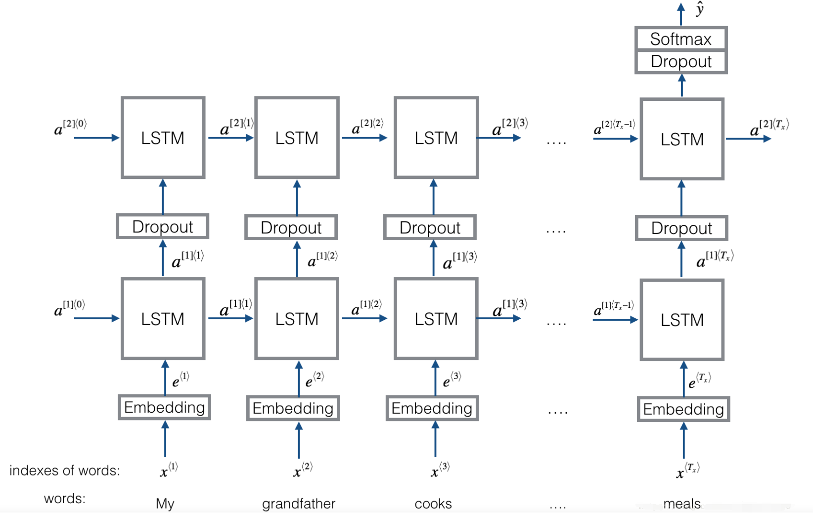
embedding层我们已经构建完成了,现在我们将它的输出输入到LSTM中。
模型的输入是(m, max_len),定义在了input_shape中,输出是(m, C=5)
def Emojify_V2(input_shape, word_to_vec_map, word_to_index):
    """
    实现Emojify-V2模型的计算图

    参数:
        input_shape -- 输入的维度,通常是(max_len,)
        word_to_vec_map -- 字典类型的单词与词嵌入的映射。
        word_to_index -- 字典类型的单词到词汇表(400,001个单词)的索引的映射。

    返回:
        model -- Keras模型实体
    """
    # 定义sentence_indices为计算图的输入,维度为(input_shape,),类型为dtype 'int32'
    sentence_indices = Input(input_shape, dtype='int32')

    # 创建embedding层
    embedding_layer = pretrained_embedding_layer(word_to_vec_map, word_to_index)

    # 通过嵌入层传播sentence_indices,你会得到嵌入的结果
    embeddings = embedding_layer(sentence_indices)

    # 通过带有128维隐藏状态的LSTM层传播嵌入
    # 需要注意的是,返回的输出应该是一批序列。
    X = LSTM(128, return_sequences=True)(embeddings)
    # 使用dropout,概率为0.5
    X = Dropout(0.5)(X)
    # 通过另一个128维隐藏状态的LSTM层传播X
    # 注意,返回的输出应该是单个隐藏状态,而不是一组序列。
    X = LSTM(128, return_sequences=False)(X)
    # 使用dropout,概率为0.5
    X = Dropout(0.5)(X)
    # 通过softmax激活的Dense层传播X,得到一批5维向量。
    X = Dense(5)(X)
    # 添加softmax激活
    X = Activation('softmax')(X)

    # 创建模型实体
    model = Model(inputs=sentence_indices, outputs=X)

    return model
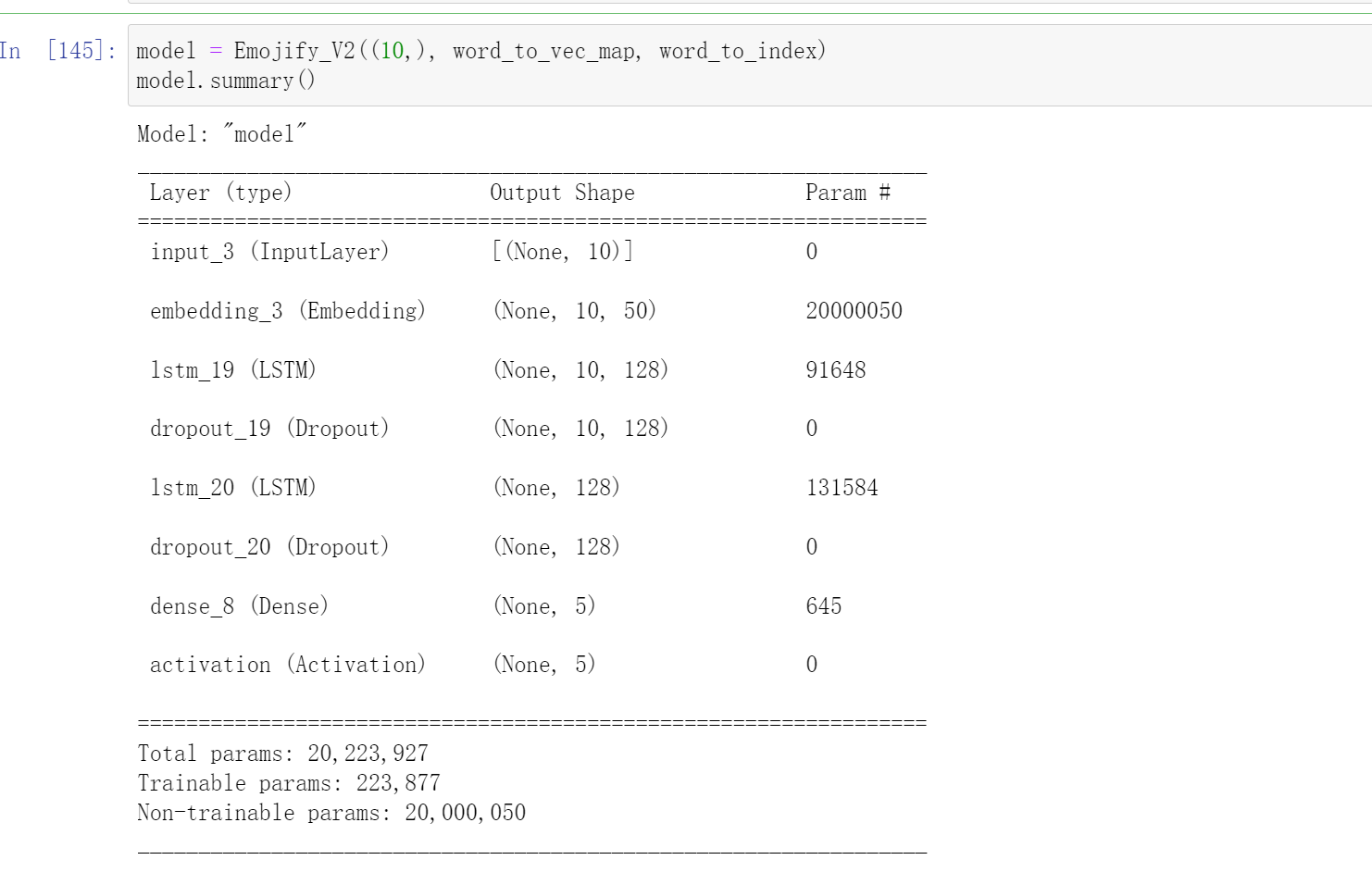
因为数据集中所有句子都小于10个单词,所以我们选择max_len=10。在接下来的代码中,你应该可以看到有“20,223,927”个参数,其中“20,000,050”个参数没有被训练(这是因为它是词向量),剩下的是有“223,877”被训练了的。因为我们的单词表有400,001个单词,所以是400 , 001 ∗ 50 = 20 , 000 , 050 400,001*50=20,000,050400,001∗50=20,000,050个不可训练的参数。
model = Emojify_V2((max_Len,), word_to_vec_map, word_to_index)
model.summary()
model.compile(loss='categorical_crossentropy', optimizer='adam', metrics=['accuracy'])
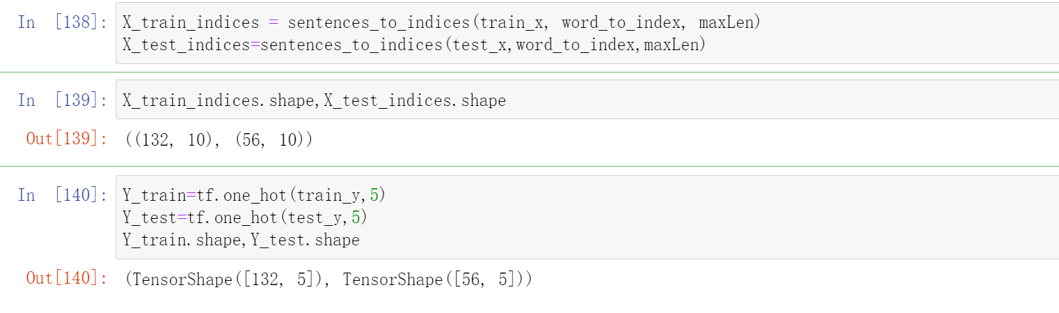
由于我们的模型是以(m, max_len)为输入,(m, number of classes)为输出。在训练之前,我们还需要把train和test数据弄好
X_train_indices = sentences_to_indices(train_x, word_to_index, maxLen)
X_test_indices=sentences_to_indices(test_x,word_to_index,maxLen)

Y_train=tf.one_hot(train_y,5)
Y_test=tf.one_hot(test_y,5)
Y_train.shape,Y_test.shape
然后开始训练
epochs = 100
batch_size = 32
history = model.fit(X_train_indices, Y_train, epochs=epochs, batch_size=batch_size,
        validation_data=(X_test_indices, Y_test))
-----
Epoch 96/100
5/5 [==============================] - 0s 12ms/step - loss: 0.0018 - accuracy: 1.0000 - val_loss: 0.6327 - val_accuracy: 0.8214
Epoch 97/100
5/5 [==============================] - 0s 12ms/step - loss: 0.0026 - accuracy: 1.0000 - val_loss: 0.6460 - val_accuracy: 0.8214
Epoch 98/100
5/5 [==============================] - 0s 12ms/step - loss: 0.0031 - accuracy: 1.0000 - val_loss: 0.6801 - val_accuracy: 0.8393
Epoch 99/100
5/5 [==============================] - 0s 14ms/step - loss: 0.0018 - accuracy: 1.0000 - val_loss: 0.7120 - val_accuracy: 0.8393
Epoch 100/100
5/5 [==============================] - 0s 13ms/step - loss: 0.0039 - accuracy: 1.0000 - val_loss: 0.7733 - val_accuracy: 0.8214
3 将输入改变的另一种方式
上面是大多数博客中写到的。在这个嵌入层( The Embedding layer)中
Embedding 层。这个例子展示了两个样本通过embedding层,两个样本都经过了max_len=5的填充处理,最终的维度就变成了(2, max_len, 50),这是因为使用了50维的词嵌入。
所以我们为何不直接将模型的输入改成(batch size, max input length, dimension of word vectors),这里就是(batch size,10,50).
代码:
- 加载向量
def read_glove_vecs(glove_file):
    with open(glove_file, 'r', encoding='utf8') as f:
        words = set()
        word_to_vec_map = {}
        for line in f:
            line = line.strip().split()
            curr_word = line[0]
            words.add(curr_word)
            word_to_vec_map[curr_word] = np.array(line[1:], dtype=np.float64)

        i = 1
        words_to_index = {}
        index_to_words = {}
        for w in sorted(words):
            words_to_index[w] = i
            index_to_words[i] = w
            i = i + 1
    return words_to_index, index_to_words, word_to_vec_map
word_to_index, index_to_word, word_to_vec_map = read_glove_vecs('data/glove.6B.50d.txt')
- x维度变化
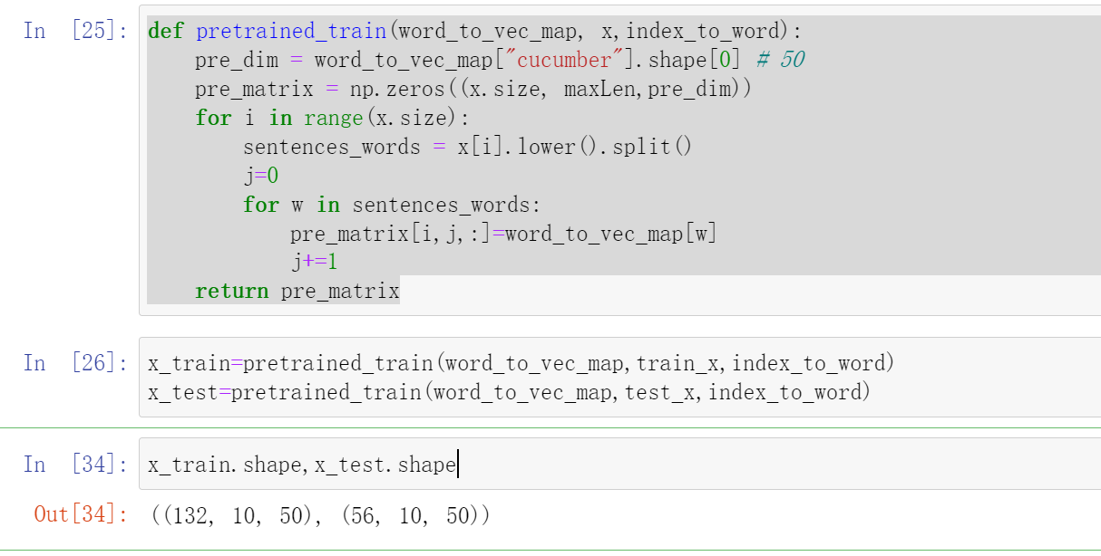
首先指定最长句子的长度,然后对其他句子进行填充到相同长度。这里我们直接初始化了一个\(pre[batch size,10,50]\)的全0的矩阵,这个矩阵\(pre[i,j,:]\)的意思就是第\(i\)个句子中第\(j\)个单词的词向量,因为在word_to_vec_map中每个单词都是用一个(50,)表示的
def pretrained_train(word_to_vec_map, x,index_to_word):
    pre_dim = word_to_vec_map["cucumber"].shape[0] # 50
    pre_matrix = np.zeros((x.size, maxLen,pre_dim))
    for i in range(x.size):
        sentences_words = x[i].lower().split()
        j=0
        for w in sentences_words:
            pre_matrix[i,j,:]=word_to_vec_map[w]
            j+=1
    return pre_matrix
x_train=pretrained_train(word_to_vec_map,train_x,index_to_word)
x_test=pretrained_train(word_to_vec_map,test_x,index_to_word)
x_train.shape,x_test.shape
- onehot转化
Y_train=tf.one_hot(train_y,5)
Y_test=tf.one_hot(test_y,5)
Y_train.shape,Y_test.shape
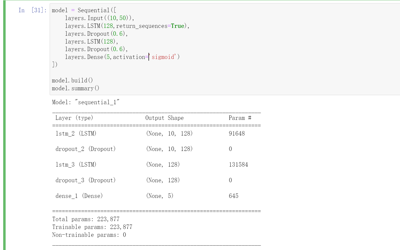
- 加载模型
model = Sequential([
    layers.Input((10,50)),
    layers.LSTM(128,return_sequences=True),
    layers.Dropout(0.6),
    layers.LSTM(128),
    layers.Dropout(0.6),
    layers.Dense(5,activation='sigmoid')
])

model.build()
model.summary()
model.compile(loss='categorical_crossentropy', optimizer='adam', metrics=['accuracy'])
epochs = 100
batch_size = 32
history = model.fit(x_train, Y_train, epochs=epochs, batch_size=batch_size,
        validation_data=(x_test, Y_test))
Epoch 95/100
5/5 [==============================] - 0s 15ms/step - loss: 0.0057 - accuracy: 1.0000 - val_loss: 0.4291 - val_accuracy: 0.8929
Epoch 96/100
5/5 [==============================] - 0s 15ms/step - loss: 0.0047 - accuracy: 1.0000 - val_loss: 0.4401 - val_accuracy: 0.9107
Epoch 97/100
5/5 [==============================] - 0s 15ms/step - loss: 0.0077 - accuracy: 1.0000 - val_loss: 0.4580 - val_accuracy: 0.9107
Epoch 98/100
5/5 [==============================] - 0s 14ms/step - loss: 0.0075 - accuracy: 1.0000 - val_loss: 0.4518 - val_accuracy: 0.9107
Epoch 99/100
5/5 [==============================] - 0s 15ms/step - loss: 0.0052 - accuracy: 1.0000 - val_loss: 0.4298 - val_accuracy: 0.9107
Epoch 100/100
5/5 [==============================] - 0s 16ms/step - loss: 0.0044 - accuracy: 1.0000 - val_loss: 0.4043 - val_accuracy: 0.9107
然后我们来测试一下吧:
test = np.array(['you are so beautiful'])
test_indices = pretrained_train(word_to_vec_map,test,index_to_word)
print(test[0] +' '+  label_to_emoji(np.argmax(model.predict(test_indices))))
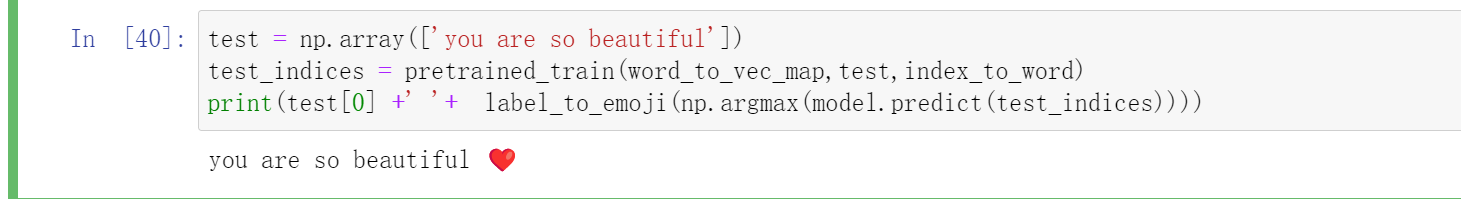
训练集比较小,如果训练集比较大的话LSTM就会表现的更好。