博客地址:https://www.cnblogs.com/zylyehuo/
1、【MATLAB绘图】绘制对应曲线图,在legend图注处标明对应曲线的w_n、zeta取值;高阶零极点的数值;
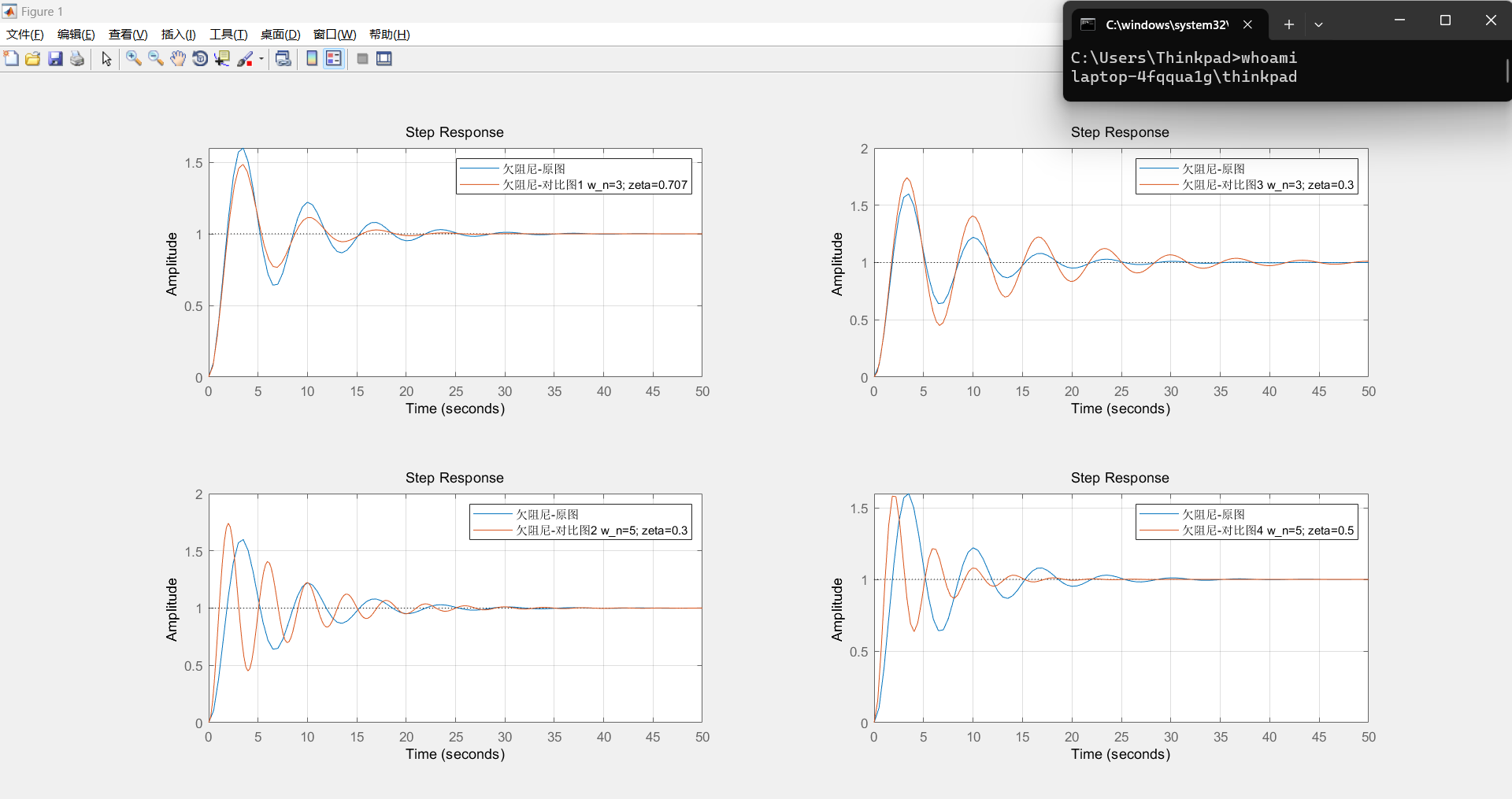
绘制4张欠阻尼二阶系统不同系数变化下的对比图,观察四种变化造成的单位阶跃响应的变化
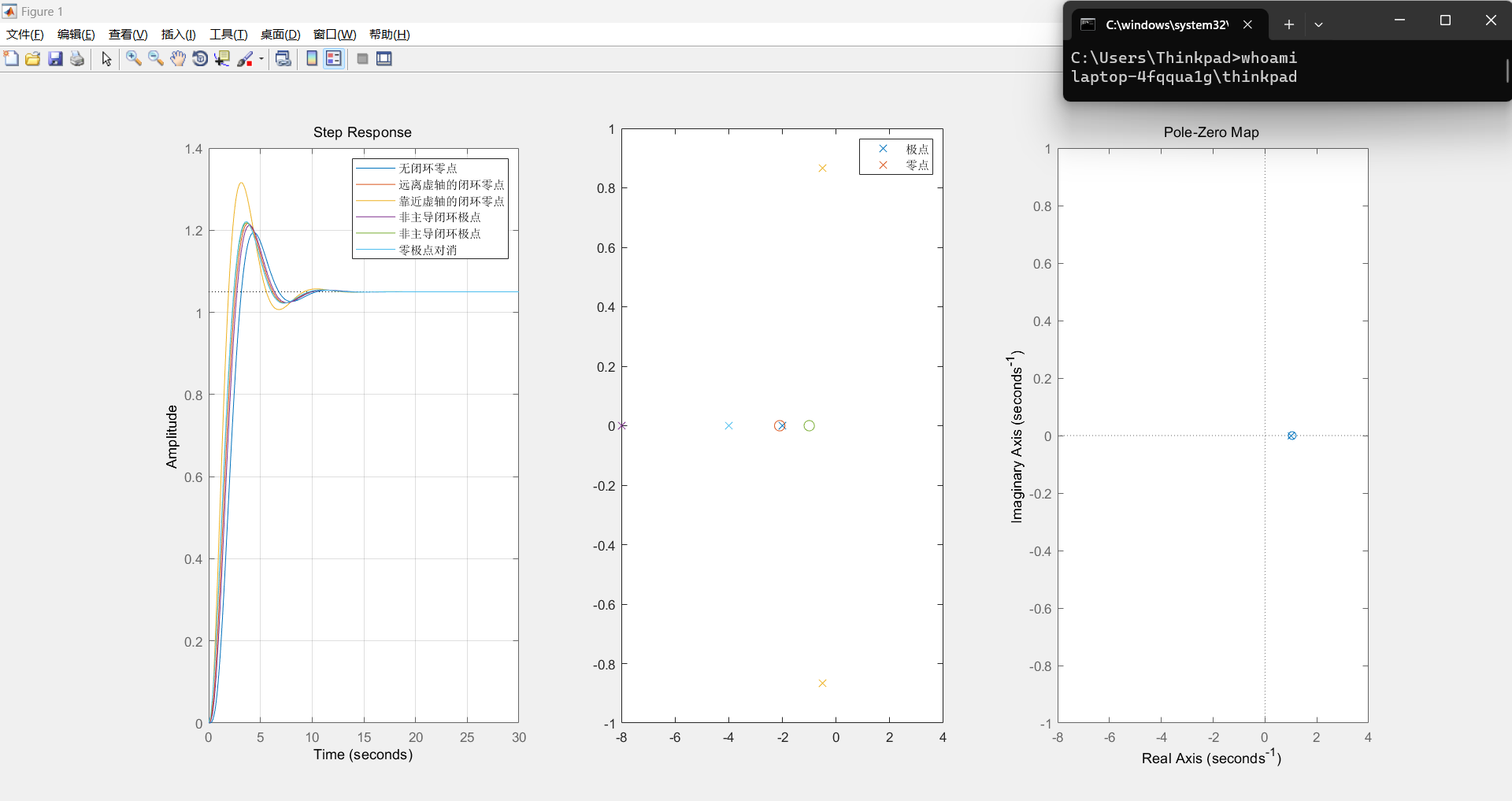
绘制高阶系统对比图,观察零极点变化下的单位阶跃响应的区别
- !
2、【文字描述】对比分析各曲线图中参数、零极点配置等变化时,对系统的影响;
4张欠阻尼二阶系统不同系数变化下的对比图
- w_n越大,t_p越小,t_s越小,超调量越小
- zeta越小,t_p越大,t_s越大,超调量越大
高阶系统对比图
- 闭环零点:减少峰值时间,减缓系统响应速度,增大超调量,等价于减小系统阻尼;
- 如果系统存在极点位于右半平面或存在多个极点位于虚轴上,那么系统就是不稳定的;
- 零点可以起到稳定化系统的作用,当零点和极点相互抵消时,可以使系统更加稳定;
- 极点会对系统的响应速度、稳态误差以及超调量等产生影响。
3. 【MATLAB代码】附全部代码。
demo01.m
clc;
clear;
close all;
w_n=3;
w_n0=3;
w_n1=5;
w_n2=3;
w_n3=5;
t_final=50;
zeta=0.5;G_2order = tf([w_n^2],[10 2*zeta*w_n w_n^2]);
zeta=0.707;G_2order0 = tf([w_n0^2],[10 2*zeta*w_n0 w_n0^2]);
zeta=0.3;G_2order1 = tf([w_n1^2],[10 2*zeta*w_n1 w_n1^2]);
zeta=0.3;G_2order2 = tf([w_n2^2],[10 2*zeta*w_n2 w_n2^2]);
zeta=0.5;G_2order3 = tf([w_n3^2],[10 2*zeta*w_n3 w_n3^2]);

figure;
subplot(2,2,1);step(G_2order,G_2order0,t_final);grid on;hold on;legend('欠阻尼-原图','欠阻尼-对比图1 w_n=3; zeta=0.707');
subplot(2,2,3);step(G_2order,G_2order1,t_final);grid on;hold on;legend('欠阻尼-原图','欠阻尼-对比图2 w_n=5; zeta=0.3');
subplot(2,2,2);step(G_2order,G_2order2,t_final);grid on;hold on;legend('欠阻尼-原图','欠阻尼-对比图3 w_n=3; zeta=0.3');
subplot(2,2,4);step(G_2order,G_2order3,t_final);grid on;hold on;legend('欠阻尼-原图','欠阻尼-对比图4 w_n=5; zeta=0.5');
demo02.m
clc;
clear;
close all;

w_n=4;
t_final=30;
zeta=0.2;

num1 = [1.05];
den1 = [1,1,1];
sys1 = tf(num1,den1);

num2 = [1];
den2 = [0.5,1];
sys2 = tf(num2,den2);

num3 = [1];
den3 = [0.125,1];
sys3 = tf(num3,den3);

sys4 = series(sys1,sys2);

num5 = [0.4762,1];
den5 = [1];
sys5 = tf(num5,den5);

num6 = [1,1];
den6 = [1];
sys6 = tf(num6,den6);

[num4,den4] = series(num1,den1,num2,den2);
[num,den] = series(num3,den3,num4,den4);

num8 = [1];
den8 = [0.25,1];
sys10 = tf(num8,den8);
sys11 = series(sys4,sys5);

sys7 = series(sys3,sys4);
sys8 = series(sys5,sys7);
sys9 = series(sys6,sys7);
sys12 = series(sys10,sys11);

% 无闭环零点
ps=roots(num);
zs=roots(den);
subplot(132);
plot(real(zs),imag(zs),'x',real(ps),imag(ps),'o','markersize',8);
axis([-8,4,-1,1]);
grid;%绘制网格线
hold on;
legend('极点','零点');
subplot(133);
pzmap(den,num);
axis([-8,4,-1,1]);
hold on;

% 远离虚轴的闭环零点
[num8, den8] = tfdata(sys8, 'v');
ps=roots(num8);
zs=roots(den8);
subplot(132);
plot(real(zs),imag(zs),'x',real(ps),imag(ps),'o','markersize',8);
axis([-8,4,-1,1]);
grid;%绘制网格线
hold on;
legend('极点','零点');
subplot(133);
pzmap(den8,num8);
axis([-8,4,-1,1]);
hold on;

% 靠近虚轴的闭环零点
[num9, den9] = tfdata(sys9, 'v');
ps=roots(num9);
zs=roots(den9);
subplot(132);
plot(real(zs),imag(zs),'x',real(ps),imag(ps),'o','markersize',8);
axis([-8,4,-1,1]);
grid;%绘制网格线
hold on;
legend('极点','零点');
subplot(133);
pzmap(den9,num9);
axis([-8,4,-1,1]);
hold on;

% 非主导闭环极点
[num12, den12] = tfdata(sys12, 'v');
ps=roots(num12);
zs=roots(den12);
subplot(132);
plot(real(zs),imag(zs),'x',real(ps),imag(ps),'o','markersize',8);
axis([-8,4,-1,1]);
grid;%绘制网格线
hold on;
legend('极点','零点');
subplot(133);
pzmap(den12,num12);
axis([-8,4,-1,1]);
hold on;

% 非主导闭环极点
[num11, den11] = tfdata(sys11, 'v');
ps=roots(num11);
zs=roots(den11);
subplot(132);
plot(real(zs),imag(zs),'x',real(ps),imag(ps),'o','markersize',8);
axis([-8,4,-1,1]);
grid;%绘制网格线
hold on;
legend('极点','零点');
subplot(133);
pzmap(den11,num11);
axis([-8,4,-1,1]);
hold on;

% 零极点对消
ps=roots(num1);
zs=roots(den1);
subplot(132);
plot(real(zs),imag(zs),'x',real(ps),imag(ps),'o','markersize',8);
axis([-8,4,-1,1]);
grid;%绘制网格线
hold on;
legend('极点','零点');
subplot(133);
pzmap(den1,num1);
axis([-8,4,-1,1]);
hold on;

G_2order0 = sys7;%无闭环零点
G_2order1 = sys8;%远离虚轴的闭环零点
G_2order2 = sys9;%靠近虚轴的闭环零点
G_2order3 = sys12;%非主导闭环极点
G_2order4 = sys11;%非主导闭环极点
G_2order5 = sys1;%零极点对消

subplot(1,3,1);step(G_2order0,G_2order1,G_2order2,G_2order3,G_2order4,G_2order5,t_final);grid on;hold on;legend('无闭环零点','远离虚轴的闭环零点','靠近虚轴的闭环零点','非主导闭环极点','非主导闭环极点','零极点对消');